Term Frequency - Inverse Document Frequency

Descrbing a document by its words

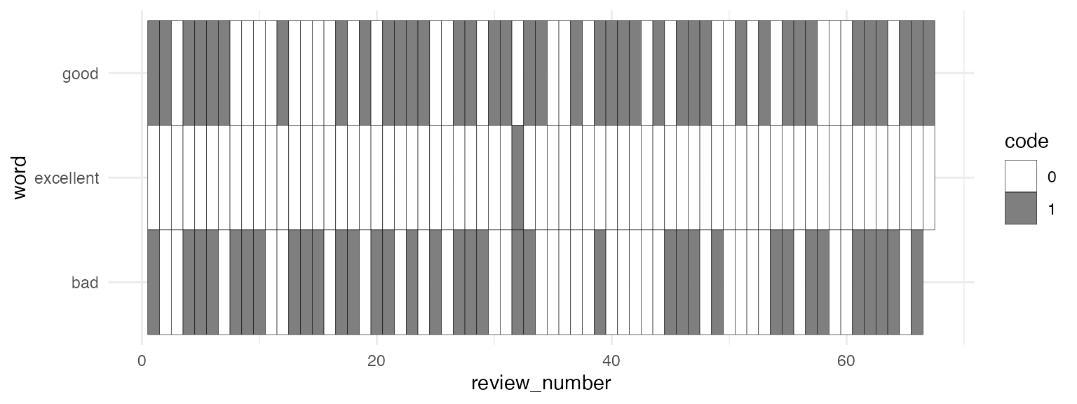
Binary coding

One way to represent the content of a document, like a movie review, is with a binary code of 1, if a word appears in it, or a 0, if a word does not.

python

import numpy as np

import nltk
from nltk.corpus import movie_reviews
from nltk.corpus import stopwords
all_ids = movie_reviews.fileids()
all_words = [movie_reviews.words(id) for id in all_ids]

python

english_stop = stopwords.words("english")
print(english_stop[0:10])

['i', 'me', 'my', 'myself', 'we', 'our', 'ours', 'ourselves', 'you', "you're"]

python

all_words_filtered = [
  [
    word 
    for word in review 
    if word not in english_stop
  ]
  for review in all_words
]

python

review_has_good = np.array([
  1 
  if "good" in review
  else
  0
  for review in all_words_filtered
])

review_has_excellent = np.array([
  1 
  if "excellent" in review
  else
  0
  for review in all_words_filtered
])

review_has_bad = np.array([
  1 
  if "bad" in review
  else
  0
  for review in all_words_filtered
])

Figure 1: Presence or absence of ‘good’ and ‘bad’

Token Counts

Or, we could count how often each word appeared in a review. Probably if a review has the word “good” in it 6 times, that’s a more important word to the review than one where it appears just once.

python

from collections import Counter

good_count = np.array([
  Counter(review)["good"]
  for review in all_words_filtered
])

excellent_count = np.array([
  Counter(review)["excellent"]
  for review in all_words_filtered
])

bad_count = np.array([
  Counter(review)["bad"]
  for review in all_words_filtered
])

Since the reviews are different lengths, we can “normalize” them.

python

total_review = np.array([
  len(review)
  for review in all_words_filtered
])

good_norm = good_count/total_review
excellent_norm = excellent_count/total_review
bad_norm = bad_count/total_review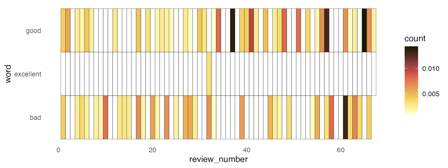

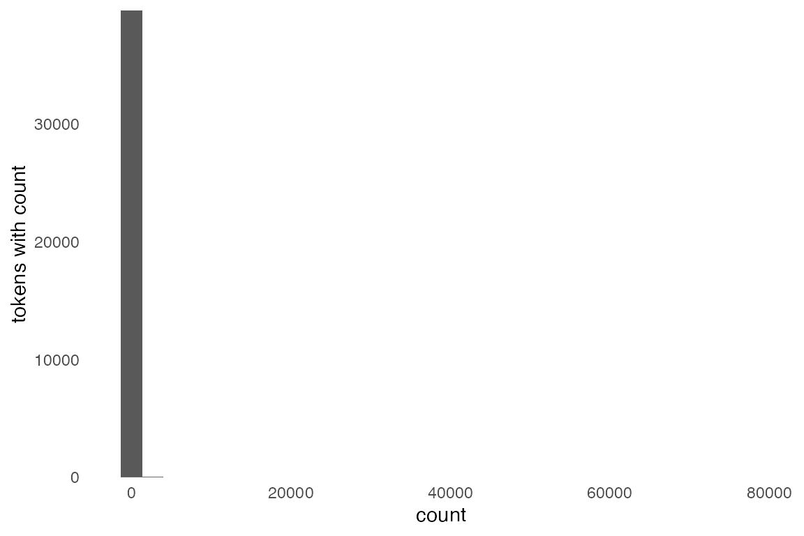
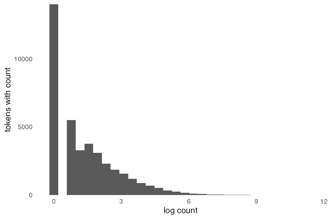
Figure 2: Presence or absence of ‘good’ and ‘bad’

Document Frequency

On the other hand, it looks like “good” and “bad” appear in lots of reviews.

python

review_has_good.mean()

0.591

python

review_has_bad.mean()

0.3865

Wheras, the word “excellent” doesn’t appear in that many reviews overall.

python

review_has_excellent.mean()

0.0725

Maybe, when the word “excellent” appears in a review, it should be taken more seriously, since it doesn’t appear in that many.

TF-IDF

TF

Term Frequency

IDF

Inverse Document Frequency

The TF-IDF value tries to describe the words that appear in a document by how important they are to that document.

If a word appears __ in this document	that appears in documents __	then…
often	rarely	it’s probably important
often	very often	it might not be that important

Term Frequency

\[ tf = \log C(w)+1 \]

Why log?

Figure 3: Raw Count

Figure 4: Raw Count

python

good_tf = np.log(good_count+1)
excellent_tf = np.log(excellent_count + 1)
bad_tf = np.log(bad_count + 1)

Inverse Document Frequency

If \(n\) is the total number of documents there are, and \(df\) is the number of documents a word appears in

\[ idf = \log \frac{n}{df} \]

python

n_documents = len(all_words_filtered)

good_idf = np.log(
  n_documents/review_has_good.sum()
  )

excellent_idf = np.log(
  n_documents/review_has_excellent.sum()
  )

bad_idf = np.log(
  n_documents/review_has_bad.sum()
  )

TF-IDF

We just multiply these two together

python

good_tf_idf = good_tf * good_idf
excellent_tf_idf = excellent_tf * excellent_idf
bad_tf_idf = bad_tf * bad_idf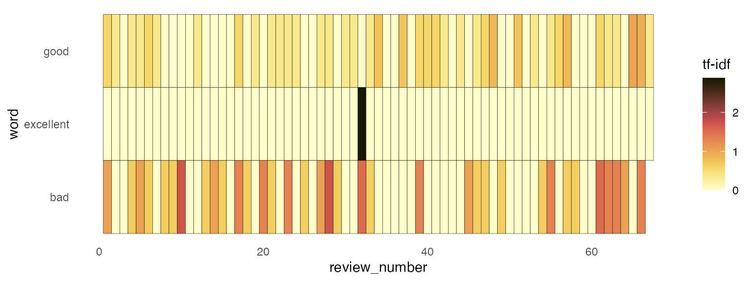

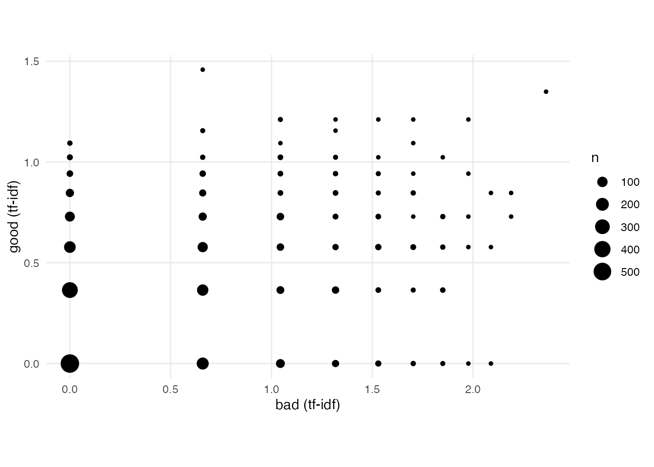
Figure 5: TF-IDF

Document “vectors”

Another way to look at these reviews is as “vectors”, or rows of numbers, that exist along the “good” axis, or the “bad” axis.

Figure 6: Documents in ‘good’ and ‘bad’ space

Doing it with sklearn

python

from sklearn.linear_model import LogisticRegression
from sklearn.model_selection import train_test_split
from sklearn.feature_extraction.text import TfidfVectorizer

Setting up the data.

python

raw_reviews = [
  movie_reviews.raw(id) 
  for id in all_ids
  ]

labels = [
  id.split("/")[0]
  for id in all_ids
]

binary = np.array([
  1 
  if label == "pos"
  else
  0
  for label in labels
])

Test-train split

python

X_train, X_test, y_train, y_test = train_test_split(
  raw_reviews,
  binary,
  train_size = 0.8
)

Making the tf-idf “vectorizor”

python

vectorizor = TfidfVectorizer(stop_words="english")
X_train_vec = vectorizor.fit_transform(X_train)
X_test_vec = vectorizor.transform(X_test)

Fitting a logistic regression

python

model = LogisticRegression(penalty = "l2")
model.fit(X_train_vec, y_train)

LogisticRegression()

In a Jupyter environment, please rerun this cell to show the HTML representation or trust the notebook.
On GitHub, the HTML representation is unable to render, please try loading this page with nbviewer.org.

Testing the logistic regression

python

preds = model.predict(X_test_vec)

Accuracy

python

(preds == y_test).mean()

0.8425

Recall

python

recall_array = np.array([
  pred 
  for pred, label in zip(preds,y_test)
  if label == 1
])

recall_array.mean()

0.86

Precision

python

precision_array = np.array([
  label
  for pred, label in zip(preds, y_test)
  if pred == 1
])
precision_array.mean()

0.8309178743961353

F score

python

precision = precision_array.mean()
recall = recall_array.mean()

2 * ((precision * recall)/(precision + recall))

0.8452088452088452

python

tokens = vectorizor.get_feature_names_out()
tokens[model.coef_.argmax()]

'life'