Logistic Regression

Comparison

Naive Bayes

A Naive Bayes classifier tries to build a model for each class. Recall Bayes’ Theorem:

\[ P(\text{data} | \text{class)}P(\text{class}) \]

The term \(P(\text{data} | \text{class})\) is a model of the kind of data that appears in each class. When trying to do a classification task, we get back how probable the data distribution for each class.

Logistic Regression

Logistic Regression instead tries to directly estimate

\[ P(\text{class} | \text{data}) \]

Some Terminology and Math

Probabilities

Probabilities range from 0 (impossible) to 1 (guaranteed).

\[ 0 \le p \le1 \]

If something happens 2 out of every 3 times, we can calculate its probability with a fraction.

\[ p = \frac{2}{3} = 0.6\bar{6} \]

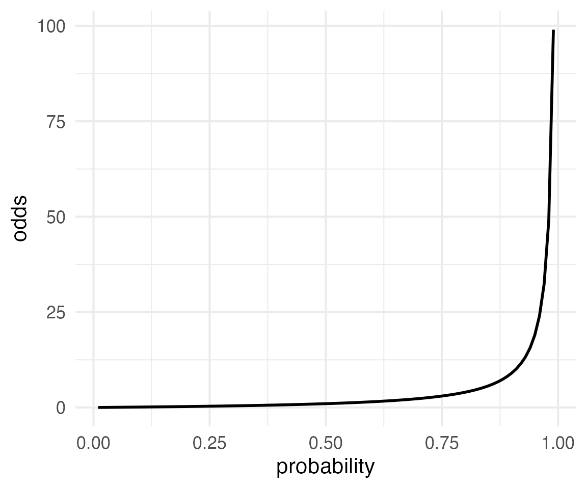
Odds

Instead of representing how often something happened out of the total possible number of times, we’d get it’s odds.

If something happens 2 out of every 3 times, that means for every 2 times it happens, 1 time it doesn’t.

\[ o = 2:1 = \frac{2}{1} = 2 \]

If we expressed the odds of the opposite outcome, it would be

\[ o = 1:2 = \frac{1}{2} = 0.5 \]

The smallest odds you can get are \(0:1\) (something never happens). The largest odds can get are \(1:0\) (something always happens). That means odds are bounded by 0 and infinity.

\[ 0 \le 0 \le \infty \]

Figure 1: The relationship between probabilities and odds

Log-Odds or Logits

The log of 0 is \(-\infty\), and the log of \(\infty\) is \(\infty\). So, if we take the log of the odds, we get a value that is symmetrically bounded.

\[ -\infty \le \log{o} \le \infty \]

Figure 2: The relationship between probabilities and logits

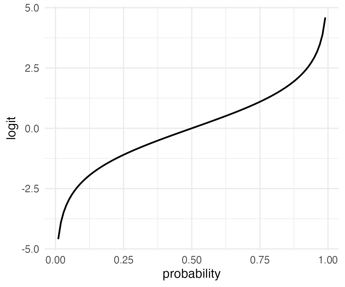
What’s also useful about this is that probabilities on opposite sides of 0.5 differ in logits only in their sign.

python

import numpy as np
from scipy.special import logit

print(logit(1/3))

-0.6931471805599454

python

print(logit(2/3))

0.6931471805599452

Why use logits?

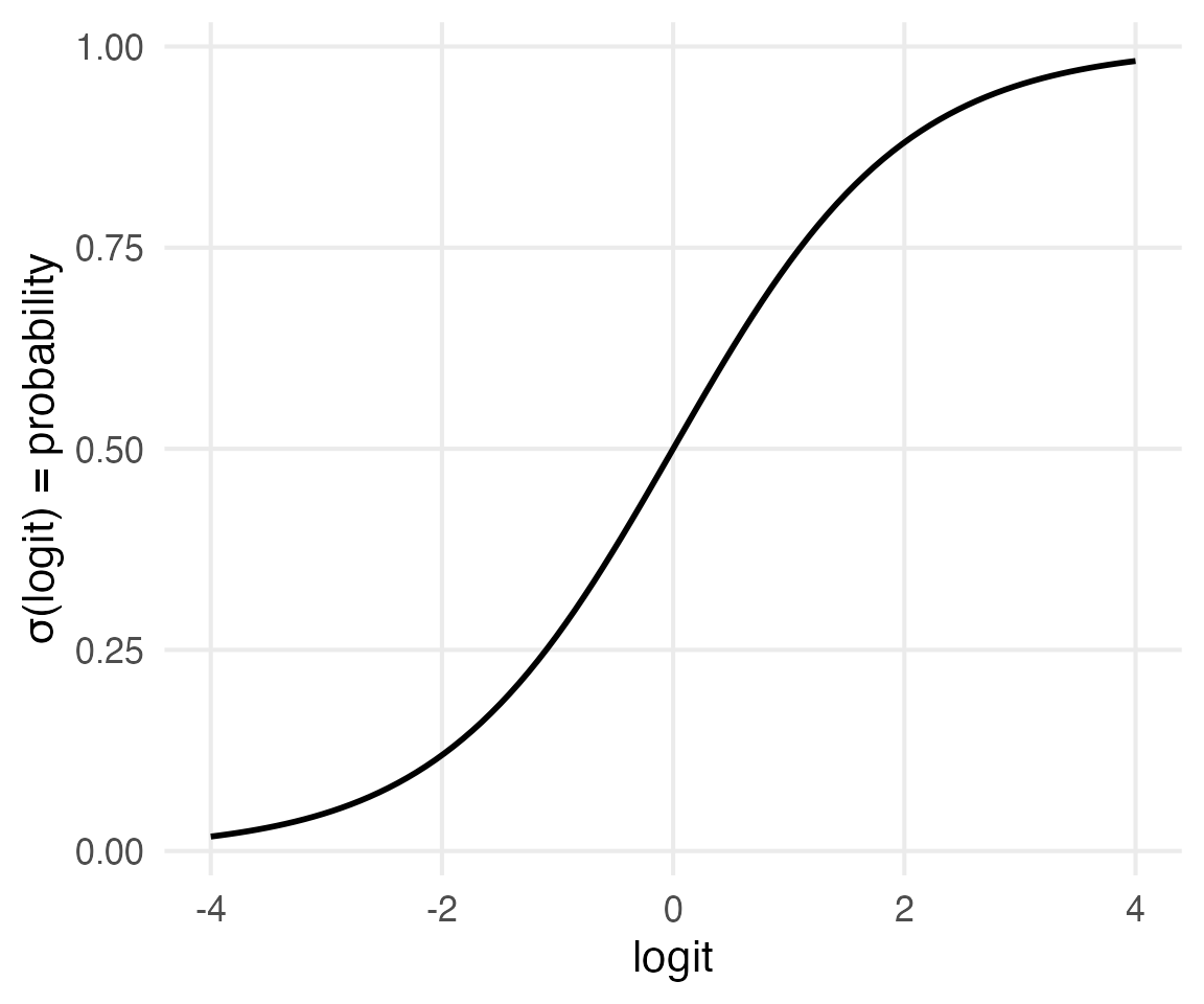
Because we can add and subtract an arbitrary number of values together (the outcome can be any negative or positive number) and then translate that back into a probability by reversing the function.

python

from scipy.special import expit
print(expit(-2))

0.11920292202211755

python

print(expit(2))

0.8807970779778823

The “inverse logit” function.

The “inverse logit” function, in NLP tasks, is usually called the “sigmoid” function, because it looks like an “S” and is represented with \(\sigma()\).

Figure 3: The σ function

Training, or Fitting, a Logistic Regression

Step 1: Deciding on your binary outcome

e.g: Positive (1) vs Negative (0) movie reviews.

Step 2: Feature engineering

You need to settle on features to encode into each training token. For example:

• How many words in the review.

• How many positive or negative words from specific sentiment lexicons.

• etc.

Step 3: “Train” the model

The model will return “weights” for each feature, and a “bias”.

• As the absolute value of weights move away from 0, you can think of that feature as being more or less important.

• As the “bias” moves up and down from 0, you can think of the overall probability moving up and down.

Figure 4: The effect of different ‘biases’ on the same set of weights.

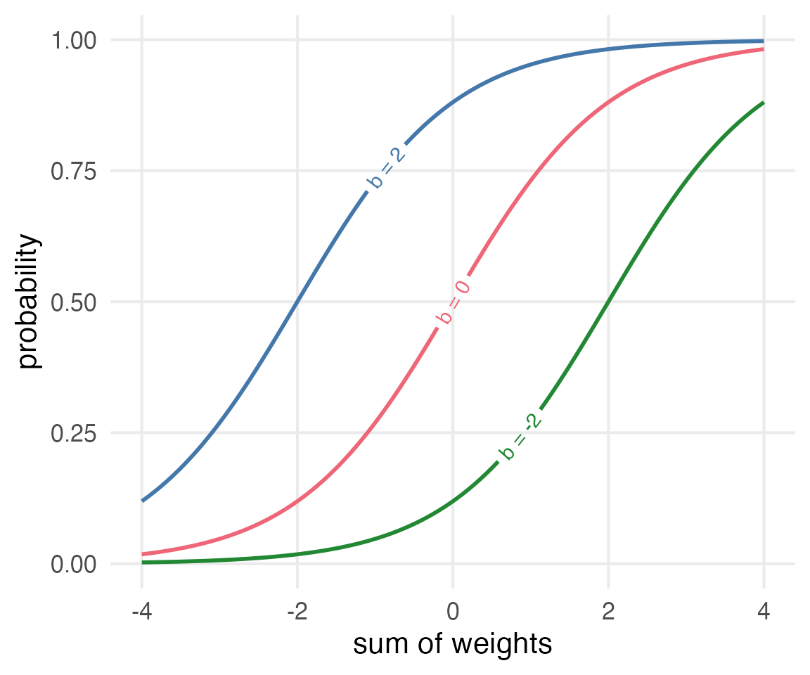
The weights

The weights we get for each feature get multiplied by the feature value, and added together to get the logit value.

\[ z = 0.5~\text{N positive words} + -0.2 ~\text{N negative words} + 0.1~\text{total length} + b \]

We could generalize the multiplication and addition:

\[ z = \left(\sum w_ix_i \right) + b \]

And, we could also even further simplify things with matrix multiplication, using the “dot product”.

\[ z = (w\cdot x) + b \]

Step 4: Use the model to classify

Now, with the features for a new set of data, multiply them by the weights, and add the bias. The categorization rule says we’ll say it’s 1 if \(\sigma(z)>0.5\), and otherwise.

\[ z' = w\cdot x' +b \]

\[ c = \left\{\begin{array}{l}1~\text{if}~\sigma(z')\gt0.5\\0~\text{otherwise} \end{array} \right\} \]

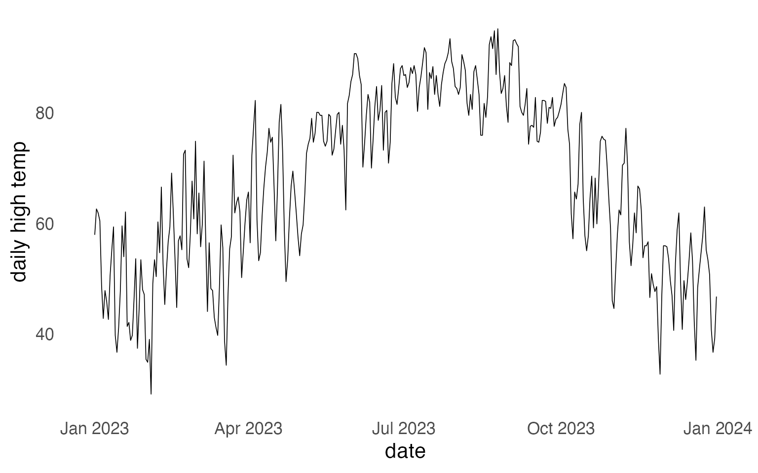
Overfitting vs Underfitting

Figure 5: Daily high temps for the Patterson Office Tower area.

Figure 6: Daily high temps for the Patterson Office Tower area.

Figure 7: Daily high temps for the Patterson Office Tower area.

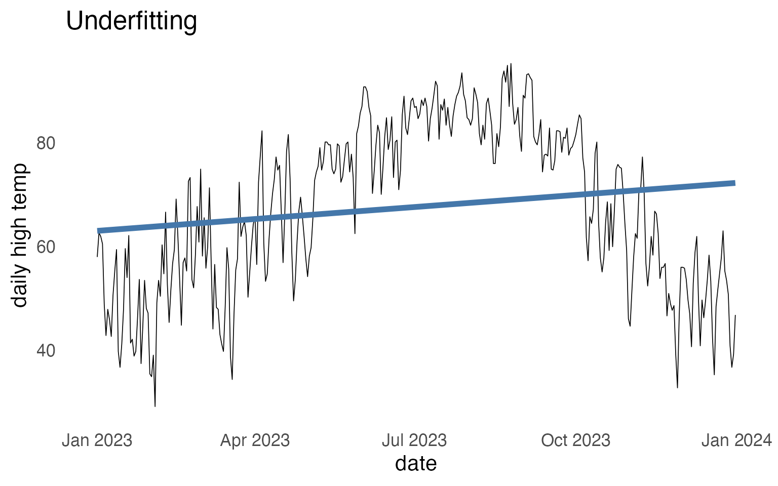
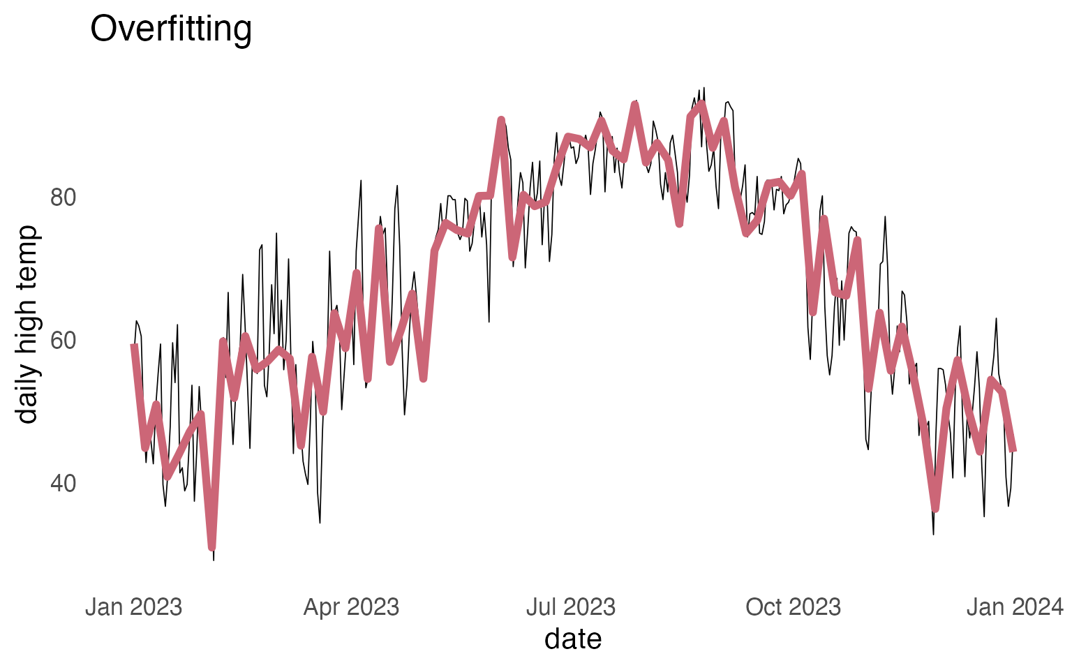
Overfitting with a classifier

If you fit a logistic regression with a ton of features, and each and every feature can get its own weight, you might “overfit” on the training data.

One way to deal with this is to try to “regularize” the estimation of weights, so that they get biased towards 0. The usual regularizing methods are (frustratingly) called “L1” and “L2” regularization.

L1 Regularization

Shrinks weights down towards 0, and may even 0 out some weights entirely.

L2 Regularization

Shrinks weights down towards 0, but probably won’t set any to exactly 0.

For ~reasons~, L2 regularization is mathematically and computationally easier to use.