Information Theory

Bits

Let’s say you live in a studio apartment. It would probably have two big-light switches. One for the main room, and one for the the bathroom. One switch has two states

1. : Off
2. : On

A single switch in a single room can give rise to two lighting conditions.

state	switches	lighting
on
off

Table 1: A single switch.

With two switches, you can have 4 unique lighting situations between the main room and the bathroom.

state_n	room	bathroom	total_lighting
1			,
2			,
3			,
4			,

Table 2: Two room lighting configurations.

If you then moved into a bigger apartment, with a separate bedroom (still open-plan kitchen+living room) that had three switches, we could have 8 different unique lighting conditions.

state_n	room	bedroom	bathroom	total_lighting
1				, ,
2				, ,
3				, ,
4				, ,
5				, ,
6				, ,
7				, ,
8				, ,

Table 3: Three room lighting configurations

I’ve put the 4 switch (16 lighting configurations) and 5 switch (32 lighting configurations) tables under these collapsible components.

4 switches

state_n	room	bedroom	kitchen	bathroom	total_lighting
1					, , ,
2					, , ,
3					, , ,
4					, , ,
5					, , ,
6					, , ,
7					, , ,
8					, , ,
9					, , ,
10					, , ,
11					, , ,
12					, , ,
13					, , ,
14					, , ,
15					, , ,
16					, , ,

5 switches

state_n	living room	dining room	bedroom	kitchen	bathroom	total_lighting
1						, , , ,
2						, , , ,
3						, , , ,
4						, , , ,
5						, , , ,
6						, , , ,
7						, , , ,
8						, , , ,
9						, , , ,
10						, , , ,
11						, , , ,
12						, , , ,
13						, , , ,
14						, , , ,
15						, , , ,
16						, , , ,
17						, , , ,
18						, , , ,
19						, , , ,
20						, , , ,
21						, , , ,
22						, , , ,
23						, , , ,
24						, , , ,
25						, , , ,
26						, , , ,
27						, , , ,
28						, , , ,
29						, , , ,
30						, , , ,
31						, , , ,
32						, , , ,

To generalize, if you have \(n\) switches, you can have \(2^n\) states.

switches	states
1	2
2	4
3	8
4	16
5	32
6	64
7	128
8	256
9	512
10	1,024

Bits → Probabilities

If someone let loose a gremlin into your \(n=3\) switch house which then randomly flipped switches, and then asked you to wager for $50 what the lighting situation was inside. You’d have to guess 1 lighting configuration out of \(2^n = 8\) possible configuration, giving you a \(\frac{1}{8} = 0.125 = 12.5\%\) chance of getting it right.

In order to represent smaller and smaller probabilities, you actually need more and more bits.

switches	states	probability
1	2	0.50000
2	4	0.25000
3	8	0.12500
4	16	0.06250
5	32	0.03125
6	64	0.01562
7	128	0.00781
8	256	0.00391
9	512	0.00195
10	1,024	0.00098

Probabilities → Bits

If we know how probable something is, can we calculate how many bits we’d need to represent it?

\[ P(x) = \frac{1}{2^n} \]

\[ P(x) = 2^{-n} \]

\[ \log_2 P(x) = -n \]

\[ -\log_2 P(x) = n \]

python

import numpy as np

# 1/8 = 0.125
-np.log2(0.125)

3.0

Abstract Bits

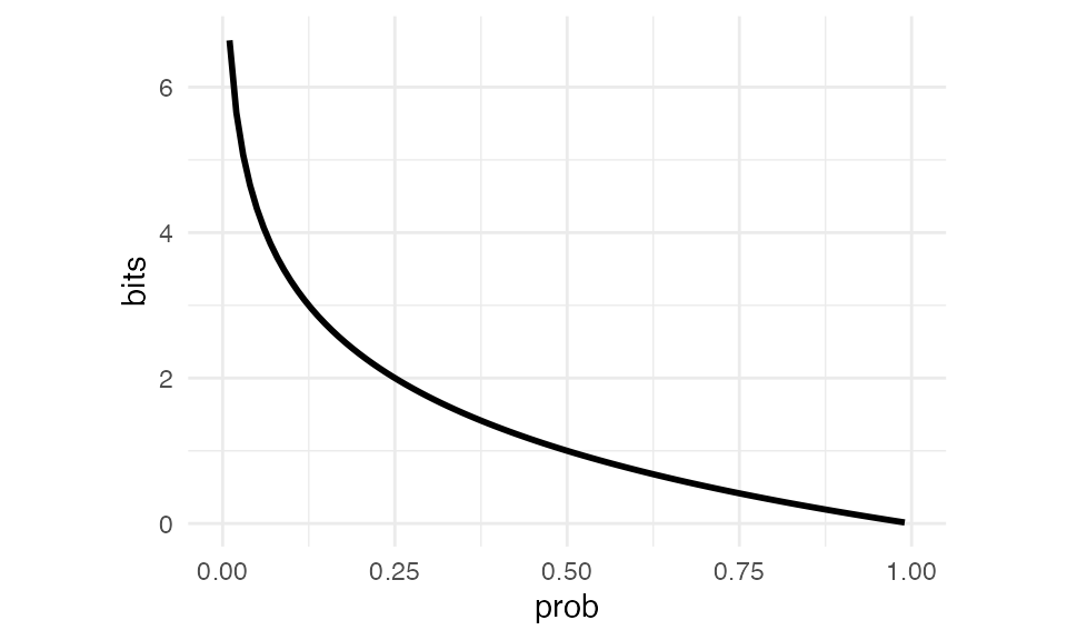
We can get more abstract, and figure out how many “bits” it takes to represent probabilities that don’t come out to whole numbers.

prob	bits
0.9	0.15
0.8	0.32
0.7	0.51
0.6	0.74
0.5	1.00
0.4	1.32
0.3	1.74
0.2	2.32
0.1	3.32

The lower the probability, the more bits we need to represent it.

Relationship between probabilities and bits

Surprisal

The term of art for “The number of bits it takes to represent a probability” is “surprisal”. Imagine I came up to you and said:

The sun rose this morning.

That’s not especially informative or surprising, since the sun rises every morning. The sun rising in the morning is a very high probability event,¹ so it’s not surprising it happens, and in the information theory world, we don’t need very many bits for it.

On the other hand, if someone came up to me and said:

The sun failed to rise this morning.

That is surprising! It’s also very informative. Thank you for telling me! I wasn’t expecting that! The smaller the probability of an event, the more surprising and informative it is if it happens, the larger the surprisal value is.

Unigram surprisal

If we get the count of every token in Moby Dick, then calculate its unigram probability, we’ll get the surprisal of every token in the book.

Relationship between probabilities and bits in unigram probabilities

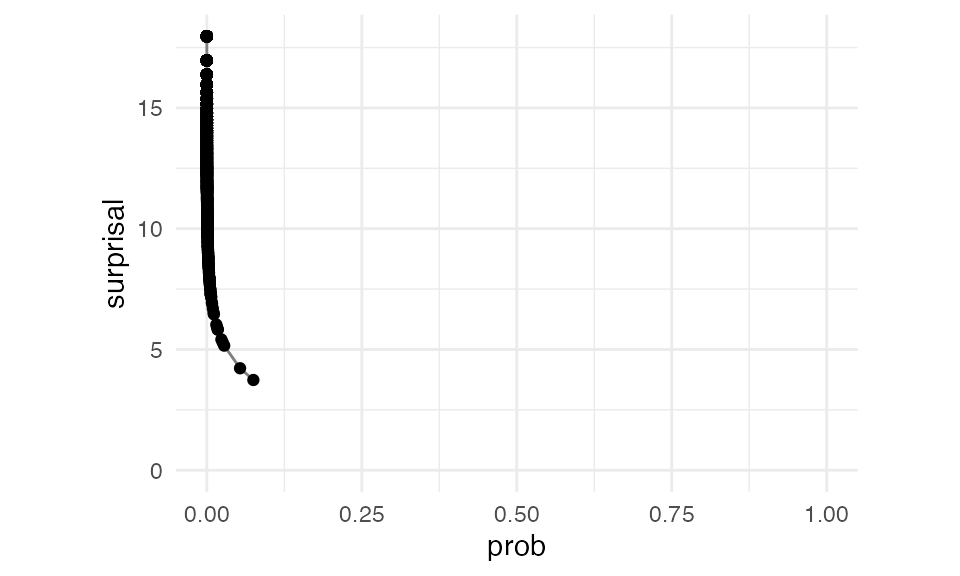
We can do this for bigrams too, looking at every \(P(w_i | w_{i-1})\).

Since a lot of \(P(w_i | w_{i-1})\) probabilities are very high, we have a lot more probabilities closer to 1, with lower surprisal, in this plot.

Entropy (or average Surprisal)

So, typically, while reading Moby Dick, how surprised, on average, are you going to be? Well, that depends on

• The surprisal of each word.

• The probability of encountering each word

\[ s(w_i) = -\log_2 P(x_i) \]

\[ H(W) = \sum_{i=1}^n P(w_i)s(w_i) = -\sum_{i=1}^n P(w_i)\log_2P(w_i) \]

	tokens	n	prob	surprisal	prob ⋅ surprisal
top 6
	,	19,211	0.34	1.57	0.53
	the	13,717	0.24	2.06	0.49
	.	7,164	0.13	3.00	0.38
	of	6,563	0.11	3.12	0.36
	and	6,009	0.11	3.25	0.34
	to	4,515	0.08	3.66	0.29
sum	—	—	—	—	2.39

If we do this for all unigrams, we get 9.66 bits.

Perplexity (or Entropy → States)

In the tokens of Moby Dick, we have 21,897 unique types.

python

from collections import Counter
moby_count = Counter(moby_dick_tokens)
len(moby_count)

21897

If each type was equally probable, our entropy would be equal to the surprisal of each token:

python

-np.log2(1/21897)

14.418445606380741

• 14.42 bits of entropy

• 21,897 states

But, with the math we did before, our average surprisal was 9.66. We could convert this actual average surprisal back states by raising it to the power of 2

python

np.exp2(9.66)

809.0023033480983

• 9.66 bits of entropy

• 809 states

How to think about Perplexity

• The actual number of states we would need in something like an FSA to capture every token in Moby Dick is 21,897

• But, the edges between nodes in that FSA are weighted.

• The degree of surprisal we experience transitioning from state to state in that FSA is like if we were using a smaller, 809 state FSA with unweighted edges.

Evalulating an ngram model.

Let’s say I had a pre-trained bigram model, and I wanted to figure out the the probability of the sentence

He saw the ship.

Our method of calculating the probability of a sentence is going to be

\[ P(w_i\dots w_{i+n}) = \prod P(w_{i+1} | w_i) \]

		prob
bigrams
	P(He|<s>)	0.021
	P(saw|He)	0.009
	P(the|saw)	0.198
	P(ship|the)	0.017
	P(.|ship)	0.069
	P(</s>|.)	0.997
prod	—	0.00000004

Very small probability, but that’s what you get when you multiply a bunch of probabilities. The total summed log-probabilities is:

python

np.array([
    lm.logscore(bg[1], [bg[0]]) 
    for bg in sent_bigram
]).sum()

-24.536868262814213

If all transitions were equally probable, we’d have

-29.986918256828176

This can be converted into an entropy:

python

lm.entropy(sent_bigram)

4.089478043802369

If we’d treated every possible transition as equally probable, we would’ve had an entropy more like:

python

-np.log2(equal_prob).mean()

7.210329710111453

And we can get the perplexity:

python

lm.perplexity(sent_bigram)

17.02376273585317

Again, if every transition had been equally probable, we’d have a perplexity of:

148.0899277945841

The upshot

The higher the probability an ngram assigns to a sentence, the lower its entropy, and the lower the perplexity.

Really novel sentences

Using the probabilities based on raw counts, we run into trouble with, say, a very novel sentence

He screamed the ship.

		prob
bigrams
	P(He|<s>)	0.021
	P(screamed|He)	0.000
	P(the|screamed)	1.000
	P(ship|the)	0.017
	P(.|ship)	0.069
	P(</s>|.)	0.997
prod	—	0

Since the sequence “He screamed” never occurred in the book, \(P(\text{screamed}|text{He}) = 0\), which means the total product of these bigrams is 0.

python

lm.entropy(sent_bigram2)

inf

python

-np.log2(0)

inf

python

target = [
  sent
  for sent in moby_words
  if "screamed" in sent
][0]

print(target[0:9])

['Wa-hee', '!', '”', 'screamed', 'the', 'Gay-Header', 'in', 'reply', ',']

Total Bigram Entropy

python

all_bigrams = [
  bg 
  for sent in moby_sents
  for bg in list(
    bigrams(
      pad_both_ends(
        word_tokenize(sent), 
        2
      )
    )
  )
]

python

lm.entropy(all_bigrams)

5.343322757138051

Footnotes

1. Depending on what latitude you live at and the time of year